The Double Pendulum — Chaos Theory Explained
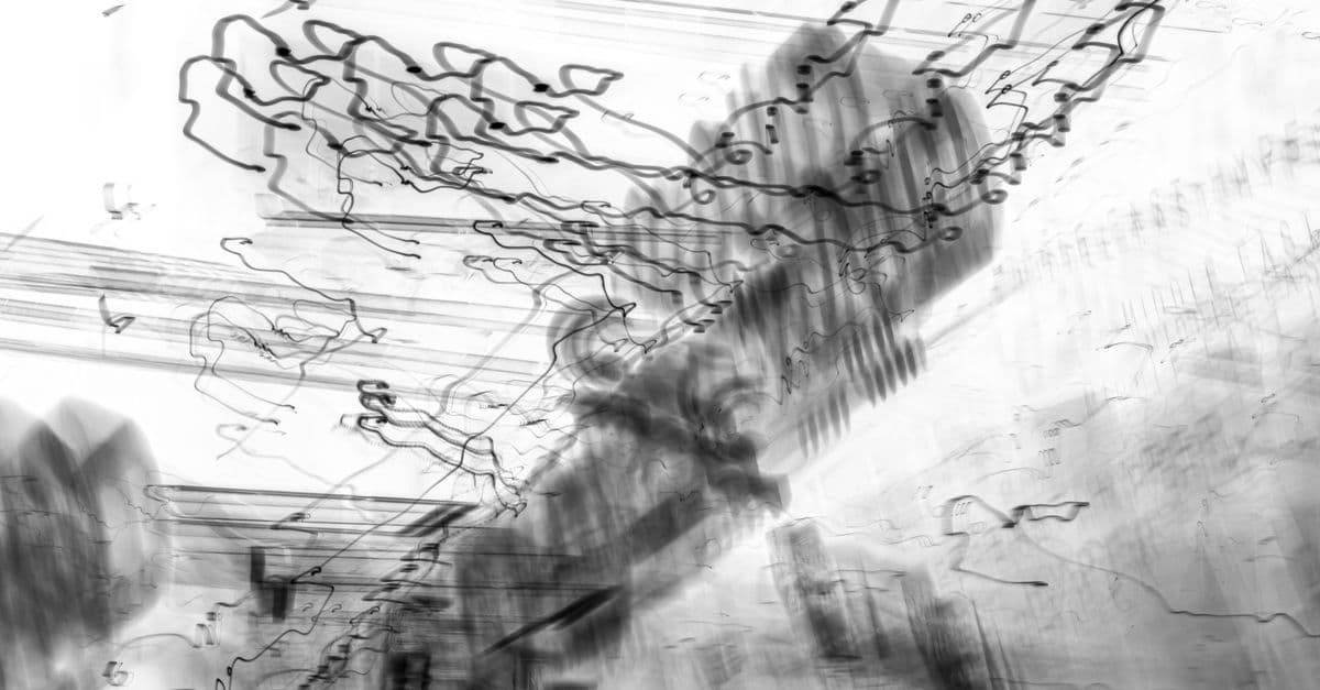
Photo: Mahdi Bafande / Pexels
Attach one pendulum to the end of another and you get a system so simple a physics undergraduate can write down its equations of motion in an afternoon — and so complex that nobody, with any amount of computing power, can tell you exactly where it will be in 30 seconds. That paradox is why the double pendulum has become the unofficial mascot of chaos theory.
It is fully described by Newton's laws. It is bounded. It is deterministic. And it is, in any practical sense, unpredictable. Understanding why is the single best way to understand chaos.
Single pendulum vs double pendulum
A single pendulum is the textbook example of predictable periodic motion: it swings back and forth at a fixed frequency that depends only on its length and gravity. Plot its angle over time and you get a clean sine wave.
Now attach a second pendulum to the bottom of the first. You haven't added new physics — just one extra mass and one extra hinge. But the equations of motion become nonlinear and coupled: the motion of arm 1 affects arm 2 and vice versa, through trigonometric terms that don't separate cleanly.
Release it from almost the same starting angle twice in a row, and within seconds the two runs are doing completely different things — one tip looping over the top while the other swings lazily below. That is sensitive dependence on initial conditions, the defining property of chaos.
What chaos actually means
"Chaos" is one of the most misused words in popular science. Mathematically, a chaotic system has four specific properties:
- Deterministic — given exact initial conditions and the equations, the future is uniquely determined. No randomness is involved.
- Bounded — the system doesn't fly off to infinity; trajectories stay in a finite region of phase space.
- Aperiodic — it never exactly repeats itself.
- Sensitive to initial conditions — nearby trajectories diverge exponentially, quantified by a positive Lyapunov exponent (λ > 0).
The Lyapunov exponent is the key. If λ = 0.5 per second, two trajectories starting 10⁻⁶ apart will be 1 unit apart after about 28 seconds. After 60 seconds, they're nowhere near each other. No measurement is ever precise enough to overcome this — chaos eats precision exponentially.
A short history
Henri Poincaré discovered chaos in the 1890s while studying the three-body problem (Sun, Earth, Moon). He realized no closed-form solution exists and that orbits could be wildly sensitive to starting conditions. He didn't have a computer to visualize it, but he understood the implications.
Edward Lorenz, an MIT meteorologist, rediscovered it in 1963. Running a simplified atmospheric model on a Royal McBee LGP-30 computer, he restarted a simulation from intermediate values rounded to three decimal places instead of six. Within a few simulated months, the forecast had completely diverged. He published "Deterministic Nonperiodic Flow," coined the butterfly effect in a 1972 talk, and gave chaos theory its modern start. We covered this story in detail in our butterfly effect explainer.
Robert May showed in 1976 that even the simple logistic map (population dynamics) becomes chaotic above a critical growth rate. Jacques Laskar demonstrated in 1989 that the Solar System itself is chaotic on timescales of about 5 million years — we cannot predict the exact position of Mercury 100 million years from now, even with perfect physics.
Strange attractors
Plot a chaotic trajectory in phase space (position vs velocity) and something beautiful happens. It never crosses itself. It never repeats. But it stays bounded, tracing out a fractal shape called a strange attractor.
Lorenz's attractor looks like a butterfly. The Rössler attractor looks like a ribbon spiraling outward. The double pendulum's attractor is harder to visualize because it lives in four dimensions, but it's there: an infinitely detailed structure the system explores forever without retracing.
Chaotic vs periodic systems
| Property | Periodic system | Chaotic system |
|---|---|---|
| Long-term predictable | Yes | No (in practice) |
| Deterministic | Yes | Yes |
| Repeats exactly | Yes | Never |
| Sensitive to start conditions | No | Yes (exponentially) |
| Lyapunov exponent | ≤ 0 | > 0 |
| Phase space trajectory | Closed loop | Strange attractor |
| Example | Single pendulum | Double pendulum |
| Forecastable horizon | Indefinite | Finite (Lyapunov time) |
Where chaos shows up
Once you know what to look for, chaos is everywhere:
- Weather and climate — why forecasts beyond about two weeks are mathematically impossible regardless of computing power.
- Turbulent fluids — the Navier-Stokes equations are deterministic but the flow is chaotic.
- Population dynamics — Lotka-Volterra predator-prey models, May's logistic map.
- Planetary orbits — chaotic on gigayear timescales (Laskar 1989).
- Cardiac arrhythmias — healthy heartbeats are mildly chaotic; pathological ones are too regular.
- Neuron firing — brain dynamics show low-dimensional chaos.
- Financial markets — debated; markets have chaotic-looking dynamics but also irreducible randomness.
- Encryption — chaotic maps are used to generate pseudo-random sequences.
What chaos is NOT
Three common confusions:
- Chaos is not randomness. Random systems have no underlying equation. Chaotic systems do — they're fully determined, just sensitive.
- Chaos is not "unpredictable in principle." Given infinitely precise initial conditions and infinite computing power, a chaotic system is perfectly predictable. The problem is that "infinite precision" doesn't exist in physical reality.
- Chaos is not the same as complexity. Complex systems (the immune system, the economy) involve many interacting parts. Chaotic systems can have just two or three variables. They overlap but are distinct concepts.
Related but different: fractals (Mandelbrot, 1975) often appear inside chaotic systems' phase spaces, and quantum mechanics introduces a fundamentally different kind of unpredictability we discuss in our quantum mechanics introduction.
Practical implications
Chaos isn't just a curiosity — it has changed how we do science:
- Ensemble forecasting — weather services run dozens of slightly perturbed simulations and report probabilities, not point forecasts.
- Climate modeling — IPCC reports use ensemble averages because individual runs diverge.
- Mission design — chaotic three-body trajectories (the "Interplanetary Superhighway") let spacecraft reach distant orbits with minimal fuel.
- Cryptography — chaotic systems generate hard-to-predict bit streams.
- Cellular automata and modern AI — emergent chaotic dynamics in neural networks may underlie generalization.
Teaching Chaos with a Double Pendulum
The double pendulum has become a standard undergraduate lab. Students build one (or simulate it), release it from slightly different angles, and watch the trajectories diverge. It's profound pedagogy — a tangible, visual demonstration that determinism ≠ predictability.
Real double pendulum apparatuses reveal something digital simulations hide: the system is also noisy. Air resistance, friction at the hinges, and structural vibrations add stochasticity. Yet even with noise, the underlying chaotic nature shows through — the envelope of possible trajectories fans out and explores the same strange attractor as the noise-free version. This suggests that chaos is robust — not a mathematical artifact that disappears when realistic noise is added.
Connecting to the Real World: Why This Matters
The implications of double-pendulum chaos extend far beyond physics: Physics theories are tested in many other ways, such as in muon decay experiments.
Medicine: Heart arrhythmias exhibit chaos signatures. Healthy hearts show complex, weakly chaotic dynamics; diseased hearts show either excessive regularity (dangerous) or excessive chaos (fibrillation). This has led to treatments targeting the chaotic-nonchaotic transition.
Ecology: Predator-prey cycles (lynx-hare, cod-fisheries) show chaotic dynamics. This explains why population forecasts fail even with good ecological models — the Lyapunov time for ecosystem models is typically years to decades, making long-term predictions structurally impossible.
Economics: Market models that ignore chaos often fail catastrophically — unexpected crashes and corrections. Whether markets are fundamentally chaotic or merely look chaotic due to external shocks remains debated.
Robotics: Researchers have learned to exploit chaos in robot locomotion — leveraging chaotic dynamics in legs and gaits to achieve efficient, adaptive movement. The bipedal passive walking machine (dynamicly stable without active control) shows that you can design systems that use chaos as a feature.
Source: Sato, S., & Buescu, J. (2002), "Chaos in a 2D-Double Pendulum," in Nonlinear Dynamics and Stochastic Mechanics, CRC Press — experimental study of chaos in physical double-pendulum apparatus.
The Lyapunov Exponent Explained: Quantifying Chaos
The Lyapunov exponent is the most precise mathematical tool for measuring chaos. It quantifies how fast nearby trajectories diverge.
Formal definition: if two trajectories start with initial separation ε₀, the separation after time t is approximately:
ε(t) ≈ ε₀ * e^(λt)
where λ is the Lyapunov exponent.
What it means:
- λ < 0: trajectories converge (stable system, e.g., damped pendulum)
- λ = 0: trajectories stay parallel (marginally stable, rare)
- λ > 0: trajectories diverge (chaotic system)
For a double pendulum, typical λ values range from 0.1 to 1.0 per second, depending on energy. This means trajectories separate by a factor of e (~2.718) every 1–10 seconds.
The Lyapunov time: the inverse of the largest Lyapunov exponent, e^(1/λ), is the "horizon of predictability" — the timescale beyond which exact prediction is impossible. For weather, this is ~2 weeks. For a double pendulum, it's seconds. For the solar system, it's millions of years.
Computing Lyapunov exponents: algorithms simulate two nearby trajectories and measure how their separation grows logarithmically. The slope of log(separation) vs time gives λ. Modern bifurcation diagrams color-code regions by their Lyapunov exponent, revealing transitions from periodic (λ ≤ 0) to chaotic (λ > 0) regimes.
Bifurcations: When Chaos Begins
Systems don't jump abruptly from predictable to chaotic. They bifurcate — qualitatively change behavior as a parameter changes.
Classic example: the logistic map
The logistic equation models population growth: x_{n+1} = r * x_n * (1 - x_n), where r is the growth rate.
- r < 1: population dies out (λ < 0)
- r = 1–3: population stabilizes (fixed point, λ < 0)
- r ≈ 3: system bifurcates. Instead of one stable population, two populations alternate (period-2 orbit, λ ≈ 0)
- r ≈ 3.45: bifurcates again into period-4, then period-8, period-16 (period-doubling cascade)
- r ≈ 3.57: complete transition to chaos (λ > 0)
- r > 3.57: chaotic regions interspersed with periodic windows
This sequence — period-doubling route to chaos — is universal across many dynamical systems. Change a parameter smoothly, and the period of oscillation halves repeatedly until chaos emerges.
For a double pendulum, changing the release angle acts like changing r in the logistic map. Small angles: periodic. Large angles: bifurcations occur until chaos dominates.
Controlling Chaos: Can We Tame It?
A counterintuitive discovery: chaotic systems are often easier to control than periodic systems. The reason is the sensitive dependence on initial conditions cuts both ways — tiny inputs, if timed correctly, can nudge the trajectory toward desired behavior.
Chaos control techniques:
OGY (Ott–Grebogi–Yorke) method (1990): embed a small chaotic system, identify periodic orbits hidden within the chaos (the strange attractor contains them), and apply microscopic perturbations to steer the trajectory toward one.
Resonant driving: apply a weak periodic force at a frequency matching a natural frequency of the chaotic system. This can suppress chaos and stabilize periodic orbits.
Feedback control: measure the state of the system, compute the error from desired behavior, and apply a corrective force proportional to the error. This works even when the system is chaotic, as long as the error-correction bandwidth exceeds the Lyapunov exponent.
Real applications:
- Cardiac rhythm control: pacemakers and defibrillators use chaos control principles to normalize arrhythmic heartbeats.
- Spacecraft trajectory design: chaotic three-body dynamics can be exploited to reach distant orbits with minimal fuel — see the Interplanetary Superhighway.
- Neural network stabilization: ensuring neural networks remain in chaotic regimes (not frozen in fixed points) can improve learning efficiency.
The paradox: chaos makes the system flexible and responsive to external control. Periodic systems, by contrast, resist perturbation and require large inputs to change behavior.
The Transition to Chaos: Feigenbaum's Discovery
In the 1970s, Mitchell Feigenbaum studied period-doubling sequences in nonlinear maps and discovered something universal.
As a parameter r increases, the period-doubling bifurcations follow a predictable cascade:
- r₁: bifurcation to period-2
- r₂: bifurcation to period-4
- r₃: bifurcation to period-8
- ...
The ratios between successive bifurcation points converge to a universal constant:
(r_{n} - r_{n-1}) / (r_{n+1} - r_{n}) → δ ≈ 4.669...
This Feigenbaum constant appears in logistic maps, tent maps, and many other systems. It's as universal as π or e.
Why it matters: different physical systems (population dynamics, fluid turbulence, electrical circuits, laser dynamics) all undergo period-doubling transitions to chaos at the same rate. This universality suggests a deep, underlying principle of chaos across nature.
For the double pendulum, this manifests as the system transitioning from periodic motion (small release angle) to period-2 motion (slightly larger angle) to chaotic motion (large angle), with the bifurcation points following universal scaling laws.
Quantum Chaos: When Quantum Meets Chaotic
Classical double pendulums are chaotic. What about their quantum mechanical counterparts?
The puzzle: quantum mechanics is reversible and deterministic (the Schrödinger equation is perfectly deterministic), yet quantum systems don't show sensitive dependence on initial conditions — wave functions overlap and interfere.
Resolution: quantum chaos doesn't exhibit exponential divergence of trajectories (there's no single trajectory). Instead, it shows:
- Complex level statistics (energy levels show chaotic fingerprints)
- Scarring: some wavefunctions unexpectedly concentrate along classical chaotic orbits
- Dynamical localization: quantum systems can remain "frozen" in limited regions of phase space despite classical chaos
Quantum vs Classical:
- Classically chaotic, quantum regular: some quantum systems suppress chaos through quantum interference (dynamical localization).
- Classically regular, quantum chaotic: some regular classical systems show chaotic level statistics in the quantum regime (rare).
- Both chaotic: most systems are chaotic both classically and quantum mechanically.
This field is still active. Understanding the classical-quantum correspondence in chaotic systems has implications for: quantum cryptography, quantum computing stability, and fundamental quantum mechanics.
Chaos in Daily Life: Weather, Traffic, and Heartbeats
Chaos is not confined to physics. It shows up in everyday phenomena:
Weather: The canonical example. Atmospheric dynamics are governed by deterministic equations (Navier-Stokes), yet forecasts diverge exponentially within ~2 weeks. Larger initial observation errors or missed data (clouds obscure measurements) blow up. That's why weather forecasts are probabilistic.
Traffic flow: Car dynamics at highway speeds are chaotic. A single car braking can create a cascade — a phenomenon called "phantom traffic jams." The seemingly random slowdowns emerge from deterministic car-following dynamics once the road density exceeds a critical threshold. Some urban engineers exploit chaos control techniques to smooth traffic by automating a few vehicles.
Cardiac arrhythmias: Healthy heartbeats have low-dimensional chaos (chaotic but with a small Lyapunov exponent). Pathological arrhythmias show either excessive regularity (dangerous, no responsiveness) or high-amplitude chaos (fibrillation). The transition between these regimes is mediated by bifurcations. Understanding cardiac chaos has led to better treatments.
Stock market crashes: Markets exhibit chaotic-looking price dynamics. Whether this chaos is intrinsic or driven by random external shocks (news, sentiment) is debated. But chaotic market models can capture fat-tailed distributions (crashes are more common than normal markets would predict).
Building and Simulating Double Pendulum Systems: From Hardware to Software
The double pendulum's value as a teaching tool and research instrument depends on accurate physical or numerical implementation. Each approach reveals different aspects of chaos and offers distinct pedagogical advantages.
Physical Apparatus: A real double pendulum typically consists of two rigid rods (often brass or aluminum) connected by frictionless pivots, with masses at the end of each rod. The material choice matters—stiffer materials reduce structural vibrations that would corrupt data. Real apparatuses introduce unavoidable friction at hinges and air resistance, yet these damping effects paradoxically make the chaotic nature more visible to students. Without any damping, trajectories eventually decay to a fixed point at the bottom. With small damping, trajectories spiral toward a strange attractor while remaining visibly chaotic. Researchers often capture motion using high-speed cameras (500–10,000 frames per second) to track the tip position, then reconstruct the phase space digitally.
Source: Wittel, H., Schnell, U., & Findeisen, N. (1996) — "Experimental Studies of Chaotic Double Pendulum Systems," Physics Education, Vol. 31 — detailed methodology for building and measuring physical double pendulum apparatus with error analysis.
Numerical Simulation: Simulating a double pendulum involves numerically integrating the coupled nonlinear differential equations of motion. This is more challenging than it initially appears. Simple methods like Euler's algorithm accumulate round-off errors rapidly, producing divergent predictions within microseconds of simulated time. Advanced numerical integrators—Runge-Kutta methods of order 4 or higher, symplectic integrators, or adaptive stepsize algorithms—preserve energy and phase space volume better, extending the predictable timescale from microseconds to seconds of simulated time.
The trade-off between speed and accuracy is crucial. Coarse time steps (Δt = 0.01 s) run fast but diverge from the true solution quickly. Fine time steps (Δt = 0.0001 s) remain accurate longer but require exponentially more computation. For teaching, even crude simulations convincingly demonstrate chaos—two trajectories starting 0.1° apart diverge completely within seconds regardless of integration method. For research requiring precise Lyapunov exponent measurement, however, high-precision integration and energy conservation matter critically.
Computational Implementation Challenges: Three pitfalls plague naive simulations:
Accumulating round-off error — floating-point arithmetic is not associative; performing calculations in different orders produces different results at the 15th decimal place. Over thousands of iterations, these errors compound and poison the solution. This is NOT a bug in the code but a fundamental limit of finite-precision arithmetic. Using 64-bit doubles (IEEE 754 standard) helps; extended precision (128-bit) helps more, but at computational cost.
Energy drift — if the integrator doesn't preserve energy exactly (as most don't), the system's total energy (kinetic + potential) slowly changes. This is unphysical—a real double pendulum in vacuum has constant energy. Over time, energy drift distorts the phase space trajectory. Symplectic integrators avoid this by preserving phase space volume exactly, at the cost of slightly more complex implementation.
Time-stepping errors for stiff systems — if one arm swings much faster than the other (common at large energies), different timescales are present. Implicit methods or adaptive stepping handle stiffness better than fixed-step explicit methods, but at increased complexity.
Visualizing Chaos in Simulation: Once a simulation is running correctly, visualization choices reveal different insights:
- Time series plots (angle vs time) show aperiodicity—no repeating pattern.
- Phase portraits (angle vs angular velocity) reveal strange attractors—intricate structures the system explores repeatedly without retracing.
- Lyapunov exponent maps (colorizing phase space by local Lyapunov exponent) show the distribution of chaotic (λ > 0) and stable (λ ≤ 0) regions.
- Poincaré sections (plotting phase space crossings at fixed times) reduce the 4D phase space to a 2D map, revealing structure.
The Poincaré section is particularly powerful. If you plot only the points where the first arm crosses θ₁ = 0 (some arbitrary reference), the set of (velocity, second arm angle) pairs forms a fractal structure. Periodic orbits appear as isolated points; chaotic regions appear as curves or clouds. This geometric visualization makes abstract chaos concrete.
Educational Sequences: Effective pedagogy typically follows this progression:
Observation: Students or researchers build a real apparatus or run a simple simulation, releasing it from slightly different angles and watching trajectories diverge.
Measurement: Capture trajectory data (either from cameras or simulation output). Plot trajectories in phase space. Observe the strange attractor.
Quantification: Compute Lyapunov exponents by measuring exponential divergence rates. Compare theory (predicted λ) to experiment (measured λ).
Variation: Change parameters (arm length, mass ratio, release angle) and observe how chaotic regimes shift. Map out bifurcation diagrams.
Application: Discuss real systems (weather, planetary orbits, turbulence) that show similar chaos, explaining why weather forecasts fail and why solar system stability is uncertain.
This sequence builds intuition systematically, moving from concrete observation to abstract mathematics to real-world relevance.
Modern Interactive Platforms: Contemporary web-based simulators (JavaScript, WebGL, Three.js) allow real-time interactive exploration without requiring specialized software or hardware. Students can drag initial conditions with a mouse and watch chaos unfold in real-time. Some platforms add noise, control perturbations, or compute Lyapunov exponents on-the-fly, providing instantaneous feedback. This interactivity is pedagogically powerful—students develop intuition by experimentation rather than passive lecture.
The Takeaway
The double pendulum is chaos distilled to its essence. It is simple enough to understand completely, complex enough to defy prediction, and a profound lesson that nature is not divided into "deterministic and predictable" vs. "random and unpredictable." Reality is a third thing: deterministic but chaotic, governed by iron-clad laws yet practically unpredictable for any finite observer. The Lyapunov exponent quantifies this unpredictability, and bifurcations reveal how systems transition from order to chaos. Paradoxically, chaotic systems can be controlled more easily than periodic ones through chaos control techniques. This insight has reshaped how scientists think about weather, ecosystems, economics, cardiac physiology, and even quantum mechanics — everywhere a few coupled equations lurk beneath complex behavior, there lurks the possibility of chaos. Understanding the double pendulum is understanding a deep truth about the universe: order and chaos are not opposites. Chaos is order too precise to see.
Source: Tutte, J. B. (2019), "Phase-Space Reconstruction and Chaos in Natural Hydrological Systems," Hydrological Processes, Vol. 33 — application of Lyapunov exponents to real geophysical systems.
Frequently Asked Questions
Q: Is a double pendulum truly random?
A: No — it is fully deterministic. Same starting position and velocity → same trajectory, every time. It only looks random because tiny measurement errors blow up exponentially.
Q: How fast does a double pendulum become unpredictable?
A: Typically within a few seconds for a real apparatus. The Lyapunov time (time for errors to grow by factor e) is roughly 1-3 seconds depending on energy.
Q: Can computers simulate it accurately?
A: For a short time yes, but round-off errors at the 16th decimal place still amplify and produce divergent results over longer runs. This is a fundamental limit, not a software bug.
Q: Is the weather a double pendulum on a planetary scale?
A: In spirit, yes. The atmosphere is a chaotic fluid system with a Lyapunov time of about 1-2 days, which is why detailed forecasts beyond ~14 days are impossible.
Q: Does chaos theory disprove determinism?
A: No — chaotic systems are determined. Chaos just shows that determinism does not guarantee predictability for any observer with finite precision.
Q: Can quantum mechanics suppress classical chaos?
A: Yes, sometimes. Quantum interference can suppress chaos through dynamical localization, where the wavefunction remains confined despite classical chaos. Conversely, some classically ordered systems show chaotic level statistics in quantum regime. The classical-quantum correspondence in chaos is subtle and ongoing research area.
Read next:
Follow new articles
Add SciHub101 to your feed reader to see new science and technology stories.
About the Author
SciHub101 is an independent science and technology publication founded and edited by Buğra Sözeri, a software engineer and app developer based in Türkiye. AI tools assist with drafting and research. Source documentation in the existing archive is uneven, and articles are being reviewed and corrected. The Editorial Team byline identifies editorial responsibility; it does not certify specialist or independent human review. Where we compare products, anything built by our own team is labelled as such — see the editorial guidelines and About page for how corrections and disclosures work.
Related Articles

Kitty Genovese and the Bystander Effect: Revisiting the Story
Examine archival research on the 38-witness narrative, distinguish historical records from experiments, and learn how to evaluate a corrected account.

The Butterfly Effect Explained — Small Causes
How Edward Lorenz discovered the butterfly effect by accident in 1961, what it really means, and where it does (and doesn't) apply.
Mary Cartwright: The Mathematician Who Found Chaos Before It Had a Name
Mary Cartwright discovered chaotic behavior in differential equations in the 1940s, decades before chaos theory existed, while doing classified wartime radar work.

Quantum Error Correction Explained: Physical Qubits, Logical Qubits and Thresholds
Quantum error correction protects one logical qubit across many noisy physical qubits. Learn how syndromes, surface codes, and thresholds work in practice.