How Do Neural Networks Work? The Architecture Behind Modern AI
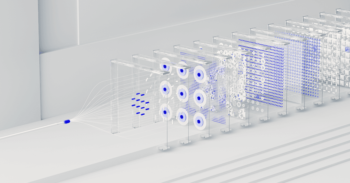
Photo: Google DeepMind / Pexels
Neural networks are the technology behind ChatGPT, image recognition, voice assistants, and most of modern AI. They're called "neural" because they were loosely inspired by biological brains, but the analogy stops there. A neural network is really a stack of mathematical functions that learn to recognise patterns in data. Once you understand the basic structure, the magic gets demystified — and the actual cleverness becomes more interesting.
Key takeaways
- A neural network is layers of artificial neurons, each performing a simple weighted sum and a non-linear transformation.
- Layers stack to learn increasingly complex patterns.
- Training adjusts the weights via backpropagation until the network's predictions match labelled data.
- Modern models have billions of parameters and learn from huge datasets.
- They're powerful but opaque — we often don't know exactly what they've learned.
What is a neural network?
A neural network has three main parts:
- Input layer — accepts the raw data (image pixels, text tokens, audio samples).
- Hidden layers — process the data through a series of transformations.
- Output layer — produces the final prediction (a classification, a number, a sequence of words).
Each layer is made of "neurons" — small computational units that combine inputs from the previous layer and pass output to the next. Information flows forward; learning flows backward.
Inside a single neuron
Each artificial neuron does three things:
- Receives inputs from many other neurons.
- Computes a weighted sum — multiplies each input by a learned weight and adds them all up, plus a bias.
- Applies an activation function — a non-linear transformation that determines the neuron's output.
The math is simple: if a neuron receives inputs x1, x2, x3 with weights w1, w2, w3 and bias b, its raw output is:
output = activation(w1*x1 + w2*x2 + w3*x3 + b)
The activation function (like ReLU: max(0, x)) is what gives the network its non-linearity — without it, stacking layers wouldn't be more powerful than a single layer. With it, the network can learn arbitrarily complex patterns given enough neurons and depth.
Why depth matters
A single layer of neurons can only learn linear patterns. Two layers can learn moderately complex patterns. Many layers ("deep" learning) can learn hierarchies of features.
In an image classifier, for example:
- Layer 1 learns to detect edges and gradients.
- Layer 2 combines edges into corners, textures, and simple shapes.
- Layer 3 combines shapes into parts (eyes, wheels, faces).
- Layer 4 combines parts into full objects (cats, cars, faces).
You don't tell the network to do this hierarchy. It emerges naturally during training. This emergent behaviour is one reason deep networks are so powerful and so hard to understand.
How training works
A neural network starts with completely random weights. Untrained, it's worse than guessing. Training is the process of adjusting those weights so the network becomes useful.
Step 1: Forward pass
Feed an example into the network. It produces a prediction (probably wrong).
Step 2: Loss calculation
Compare the prediction to the correct answer. Calculate a number — the loss — that measures how wrong the prediction was. Higher loss = more wrong.
Step 3: Backpropagation
This is the genius of neural networks. Calculate exactly how much each weight in the network contributed to the loss, by working backward from the output. Use calculus (specifically, the chain rule) to compute the gradient — the direction each weight should move to reduce loss.
Step 4: Weight update
Adjust each weight slightly in the direction that reduces loss. Just a tiny bit — typically multiplied by a small "learning rate."
Step 5: Repeat
Do this with thousands or millions of training examples, over many "epochs" (passes through the data). The weights gradually settle into a configuration that produces good predictions.
Common types of neural networks
Feedforward networks (MLPs)
The classic — neurons in fully connected layers. Good for tabular data and simple classification.
Convolutional Neural Networks (CNNs)
Designed for images. Use convolutional layers that scan across the image looking for spatial patterns. Foundational for image recognition.
Recurrent Neural Networks (RNNs) and LSTMs
Designed for sequences (text, audio, time series). They have memory — past inputs influence current outputs. Mostly superseded by transformers.
Transformers
The current state-of-the-art for most tasks. Use self-attention to weight which inputs matter most when producing an output. Power ChatGPT, Claude, Gemini, and most cutting-edge AI. The 2017 paper "Attention Is All You Need" introduced the architecture that now dominates AI.
Generative Adversarial Networks (GANs)
Two networks — a "generator" creating fake examples and a "discriminator" trying to spot them — train together. Useful for image synthesis, style transfer.
Diffusion Models
Generate images and video by learning to reverse a process of adding noise. Behind tools like DALL·E, Stable Diffusion, and Midjourney.
Why are neural networks so powerful?
Three things converged to make them dominate AI:
1. Universal approximation
Mathematically, a neural network with enough hidden neurons can approximate any continuous function. In theory, they can learn anything learnable from data.
2. Compute
Training big networks requires enormous compute. GPUs (originally for video games) turned out to be ideal — modern training runs use clusters of thousands of GPUs.
3. Data
Big networks need big data. The internet provided the corpus needed to train models on text, images, code, and more.
What we don't understand
Neural networks work astonishingly well. Why specific networks make specific decisions remains mostly opaque. This is the interpretability problem.
When a self-driving car suddenly brakes, we can examine the camera feed and the network's outputs. But understanding why the network decided to brake at that exact moment — which neurons fired, which features triggered them — is much harder. Active research areas like mechanistic interpretability try to reverse-engineer trained networks to understand their internal logic.
This matters: we deploy neural networks for medical diagnosis, hiring, lending, and parole decisions, often without knowing what they've learned.
Limitations
- Data hunger. Modern networks need huge amounts of data to learn. Humans learn from much less.
- Brittleness. Small adversarial changes to inputs can cause large output errors.
- Generalisation gap. Networks trained on one kind of data may fail on slightly different data.
- Energy cost. Training large models consumes significant electricity. GPT-4's training was estimated at 50 GWh.
- Bias. They reproduce biases in their training data.
These aren't unfixable, but they're real constraints on where neural networks should and shouldn't be deployed.
The Lottery Ticket Hypothesis and Neural Network Sparsity
A surprising discovery from recent research: most neural network parameters don't actually do anything important. The "Lottery Ticket Hypothesis" (Frankle & Carbin, 2019) proposes that when you randomly initialize a large network, a smaller subnetwork exists that, if trained in isolation, reaches comparable accuracy to the full network.
This has practical implications: pruning. Train a large network, then remove ("prune") parameters below a threshold. The remaining sparse network often performs nearly as well while being 10-100× smaller and faster.
Full network: 1 billion parameters
Train and prune: 10-50 million parameters (1% of original)
Accuracy: 95% of original
Inference speed: 10-50× faster
This explains why overparameterization works — networks are overbuilt with redundancy, but the "lottery" is the subset that matters. Finding that subset is the challenge.
Activation Functions: The Non-Linearity That Matters
We mentioned activation functions briefly, but they deserve deeper treatment. Without them, stacking layers adds no power.
ReLU (Rectified Linear Unit): max(0, x) — the modern default. Simple, fast, effective.
Sigmoid: 1 / (1 + e^-x) — older, squashes to (0, 1), used in output layers for probabilities.
Tanh: (e^x - e^-x) / (e^x + e^-x) — similar to sigmoid but output in (-1, 1).
GELU: x * Φ(x) — where Φ is the cumulative normal distribution. Smooth like tanh, but more effective at scale (used in modern transformers).
Softmax: e^xi / Σ e^xj — converts a vector to a probability distribution. Used in final layer for multi-class classification.
The choice matters. ReLU is fast; GELU is smoother and works better in large models. Sigmoid saturates (gradient → 0) for large inputs, which slows training. Modern architectures carefully select activation functions for each layer type.
The Vanishing Gradient Problem and How It's Solved
When networks get very deep (50+ layers), backpropagation multiplies gradients across many layers. If each layer's gradient is < 1, gradients exponentially shrink (vanish). If each is > 1, they exponentially explode. Both make training impossible.
Solutions:
Residual connections (ResNets): Add a skip connection that bypasses layers, allowing gradients to flow directly. This is why ResNet (He et al., 2015) was a breakthrough.
Normalization: Batch normalization, layer normalization, etc. Normalize activations to stay in a good range, stabilizing gradient flow.
Careful initialization: Initialize weights to keep gradients at scale (~1) throughout the network.
LSTM/GRU cells: Recurrent architectures designed to control gradient flow over time steps.
Modern deep networks (100+ layers) succeed because these techniques solve the vanishing gradient problem.
Regularization: Preventing Overfitting
A network trained to memorize training data won't generalize. Regularization prevents overfitting.
Dropout: Randomly drop (set to zero) units during training. Forces the network to learn redundant representations. At test time, use all units. Simple, effective, widely used.
L1/L2 regularization: Add a penalty to the loss function for large weights. Encourages the network to find small-weight solutions.
Early stopping: Monitor loss on a validation set; stop training when validation loss stops improving.
Data augmentation: Generate variations of training examples (rotate images, add noise to audio). Increases effective dataset size.
Overfitting is the #1 failure mode for neural networks on small datasets. Regularization is the defense.
Optimization Methods: From Gradient Descent to Adam
Backpropagation computes gradients, but how to adjust weights based on those gradients matters enormously.
Stochastic Gradient Descent (SGD): The simplest optimizer. After each example (or batch of examples), adjust each weight by: weight -= learning_rate × gradient. Effective but slow to converge.
Momentum: Remember the direction you were moving, and keep moving in that direction even if the gradient changes. This accelerates convergence in ravines and flat regions. SGD with momentum converges 10× faster than vanilla SGD.
Adam (Adaptive Moment Estimation): Combines momentum with adaptive per-parameter learning rates. If a parameter's gradient has been large historically, use a smaller learning rate; if small, use a larger rate. Adam is now the default optimizer for most neural network training. It's more robust than SGD to learning-rate choice and typically requires minimal tuning.
Learning rate scheduling: The learning rate (how big a step to take) affects convergence. Too high, the network overshoots optimal weights. Too low, training is agonizingly slow. Modern practice uses learning-rate schedules: start high, decay over time. Cosine annealing and warm restarts are common patterns.
The right optimizer can reduce training time by 10× or more. This matters when training takes weeks on expensive GPU clusters — getting it right saves millions in compute costs.
Source: Kingma & Ba (2014) — "Adam: A Method for Stochastic Optimization"; Ruder (2016) — "An overview of gradient descent optimization algorithms"
Transfer Learning and Fine-Tuning
Training a neural network from scratch on a new task is expensive and often fails (data-hungry networks need lots of examples). Transfer learning solves this: train a large network on a huge, diverse dataset, then adapt it to your specific task.
Pre-training: Train a model on ImageNet (14 million images, 1000 categories) or a huge text corpus (Common Crawl: 400 billion words). The model learns general-purpose features: edges, textures, simple concepts; language structure, semantics. This mirrors how language acquisition works in human brains — early learning on diverse input shapes general representations later refined for specific tasks.
Fine-tuning: Take the pre-trained model and train it on your specific task with your small dataset. Only a few layers are updated; most weights are frozen. Typically 10-100× faster and more accurate than training from scratch.
Example: A pre-trained image classifier trained on ImageNet transfers well to medical imaging (detecting tumours, pneumonia). The model has learned edges and shapes; a small amount of task-specific training adapts those features to medical images. This approach enabled rapid AI adoption in hospitals.
Few-shot and zero-shot learning: Modern large models (GPT-4, Claude) can perform new tasks with just a few examples (few-shot) or even no examples (zero-shot), given an instruction. They've learned so much from pre-training that adaptation is minimal.
Transfer learning is why large companies dominate AI — they afford the compute for pre-training on massive datasets, then all downstream applications benefit. Smaller organizations fine-tune on pre-trained models, saving enormous costs.
Source: Yosinski et al. (2014) — "How transferable are features in deep neural networks?"; Devlin et al. (2018) — BERT and transfer learning in NLP
Attention Mechanisms: The Key to Modern AI
Before transformers, most sequence models (RNNs) processed text word-by-word, left to right. Each word's representation depended on all prior words, but distant words' influence faded. Attention solved this.
Self-attention: When processing word i, look at all words in the sentence and compute a relevance score (attention weight) for each. Weight = a learned function of word i and word j. Summarize all words using these weights.
Attention(Query, Key, Value) = softmax(Q·K^T / √d_k) · V
For each position, compute three vectors from the input:
- Query: "What am I looking for?"
- Key: "What am I?"
- Value: "What information do I have?"
Attention weights (Query·Key) tell you how much each position's value to use. Modern transformers use multi-head attention — multiple sets of attention heads in parallel, each learning different relationships.
This is why transformers are so powerful: every word can directly attend to every other word in the sequence, not just prior words. Long-range dependencies are learned easily.
Cross-attention: In sequence-to-sequence models (like machine translation), the decoder attends to the encoder. This allows the output to selectively focus on relevant parts of the input.
Attention is differentiable, so gradients flow through it during training. The attention weights themselves are interpretable — you can visualize which parts of the input mattered for each output.
Source: Vaswani et al. (2017) — "Attention Is All You Need"
Scaling Laws and Emergent Behavior
A surprising discovery from training larger models: performance doesn't plateau. A model with 10 billion parameters is not just slightly better than 1 billion; it's often dramatically better.
Scaling laws (Hoffmann et al., 2022) describe this mathematically. As you scale model size N and dataset size D, loss decreases as a power law:
Loss ≈ C / N^α + C' / D^β (α ≈ 0.07, β ≈ 0.07)
Quadrupling either model size or data roughly halves the loss. This is empirically true from small models to trillion-parameter models.
Emergent abilities: Beyond raw performance, larger models exhibit qualitatively new capabilities that smaller models don't have, even if scaled down. GPT-3 (175B parameters) can do in-context learning — learn from examples in a prompt — in ways GPT-2 (1.5B) simply cannot. GPT-4 can reason about complex problems; GPT-3 struggles.
These emergent abilities are surprising because you might expect smooth improvement. Instead, some capabilities seem to "turn on" above a certain scale. The mechanisms behind this are still not well understood — active research. Understanding these phenomena requires insights from cognitive science, as researchers try to understand how learning actually works in the human brain.
Compute-optimal training: If you have a fixed compute budget, how many parameters and how much data? Chinchilla scaling laws (Hoffmann et al., 2022) show the optimal ratio: roughly equal FLOPs (floating-point operations) on parameters and data. This suggests many recent models have been under-trained on their data.
The implication: scaling isn't dead. We're not near the limit of what neural networks can do — we just need more compute, more data, and better algorithms.
Source: Hoffmann et al. (2022) — "Training Compute-Optimal Large Language Models"; Kaplan et al. (2020) — "Scaling Laws for Neural Language Models"
Neural Architecture Search: Automating Model Design
Designing neural network architectures (how many layers, how many neurons, which activation functions, etc.) was historically manual. Researchers tried architectures, ran experiments, published the best ones. This is slow and often suboptimal.
Neural architecture search (NAS) automates this: use an algorithm (reinforcement learning, evolutionary algorithms, or random search with efficient early-stopping) to explore architecture space and find high-performing designs.
Example: AutoML approaches (Google's AutoML Vision, AutoML Tables) let non-experts train competitive models. The system searches architectures, hyperparameters, and data preprocessing recipes automatically. For tabular data, this often outperforms hand-designed models.
The cost: NAS requires training thousands of candidate models, so it's compute-intensive. But when it works, it discovers architectures humans wouldn't have thought of. EfficientNet (Tan & Le, 2019) discovered models 5-10× more efficient than hand-designed ResNets by systematically scaling depth, width, and resolution.
NAS is becoming more important as models get larger (hand design doesn't scale) and deployment constraints tighten (mobile models need to be small and fast).
Source: Zoph et al. (2017) — "Learning Transferable Architectures for Scalable Image Recognition"
Frequently Asked Questions
Q: Are neural networks biologically inspired or just loosely inspired?
A: Loosely inspired at best. The basic idea of neurons and synapses led to the concept, but artificial neurons are vastly simpler than biological ones. Real neurons use chemical and electrical signaling, are asynchronous, and compute on different timescales. Artificial networks are deterministic mathematical functions on silicon — we borrowed the metaphor, not the mechanism.
Q: How large are the largest neural networks today?
A: GPT-4 has reportedly 1+ trillion parameters; Llama 3 has 70 billion. Human brains have ~86 billion neurons and ~100 trillion synapses, so largest models are in the ballpark. But parameter count doesn't map neatly to "intelligence" — it's just one dimension.
Q: Do neural networks actually think or understand language?
A: They produce outputs that look intelligent — generating coherent text, solving math problems, explaining concepts. Whether that constitutes "thinking" or "understanding" is philosophically contested. Most neuroscientists and ML researchers don't attribute consciousness to current neural networks, though this is an active debate.
Q: Why are GPUs so much faster than CPUs for neural networks?
A: Neural network training is 99% matrix multiplication. GPUs have thousands of small cores optimized for parallel matrix math (originally for graphics). A modern GPU can do 10-100× more matrix operations per second than a CPU, making them essential for training large models.
Q: Will making neural networks even larger eventually produce general intelligence?
A: Some researchers think scaling current architectures will eventually produce AGI (artificial general intelligence). Others argue we're missing something fundamental — new architectures, training methods, or physical principles. There's genuine disagreement in the field; it's an open scientific question.
Q: How does backpropagation work mathematically?
A: Backprop applies the chain rule of calculus backward through the network. For each weight, compute how much changing that weight changes the loss (the gradient). Then adjust weights in the direction that reduces loss. Repeat over millions of examples and epochs until loss plateaus. It's calculus at scale.
The bottom line
Neural networks are mathematical stacks of learned transformations. They work because stacking many layers lets them learn hierarchies of features — and because backpropagation gives us a way to adjust billions of parameters efficiently. They've gone from curiosity in the 1950s to the backbone of modern AI, powering language models, image recognition, robotics, and more. Their power comes from scale, depth, and data — but they remain partially opaque. We can train them, use them, and measure their performance, but truly understanding how and why they learn specific representations is an active research frontier.
Read next:
Follow new articles
Add SciHub101 to your feed reader to see new science and technology stories.
About the Author
SciHub101 is an independent science and technology publication founded and edited by Buğra Sözeri, a software engineer and app developer based in Türkiye. AI tools assist with drafting and research. Source documentation in the existing archive is uneven, and articles are being reviewed and corrected. The Editorial Team byline identifies editorial responsibility; it does not certify specialist or independent human review. Where we compare products, anything built by our own team is labelled as such — see the editorial guidelines and About page for how corrections and disclosures work.
Related Articles

How Does ChatGPT Actually Work? A Plain-Language Guide to LLMs
ChatGPT predicts the next word based on patterns it learned from billions of pages of text. Sounds simple — but it produces essays, code, and reasoning that look uncannily human. Here's what's really happening.
What Is Machine Learning? Explained Simply, with Real Examples
Machine learning is how computers learn patterns from data instead of being told the rules. It powers everything from email spam filters to self-driving cars. Here's how it actually works.

How Image Recognition Works: The Science of Convolutional Neural Networks
In 2010 the best image classifier missed the right label in its top five guesses about 28% of the time. By 2015 that was 3.57%. Here is what changed, and how a CNN actually sees.

How Large Language Models Work: Transformers, Attention, and Why They Hallucinate
Meta trained Llama 3 on more than 15 trillion tokens using 7.7 million H100 GPU-hours. Here is how next-token prediction at that scale turns into a conversation partner.

Edge AI: How AI Runs on Your Phone
Server-side chatbots run on racks of GPUs in data centers. Face ID, voice dictation, and a growing number of language features run on a chip the size of a fingernail in your pocket. The science of shrinking large models to fit is called edge AI.
How Diffusion Models Work: Stable Diffusion, DALL-E, and the Science of AI Art
Type a sentence, get a picture. Behind Stable Diffusion and DALL-E sits one idea borrowed from thermodynamics: destroy images with noise in small steps, train a network to undo each step, then run the process backward from static.